

How To Create A Bell Curve In Excel With Data
A bell curve, as well known as normal distribution, is the most mutual type of distribution for a variable. It is accepted every bit a distribution that occurs naturally in many situations. In a bell curve, the highest point of the arc defines the hateful, which is the highest number of occurrences of an element. The probability of occurrences decrease towards either side of the curve. Y'all can use a bell curve to compare performances by excluding extremes, or ascertain your expectations by the possibility that an consequence volition prevarication within a range to the left or right of the centre. In this guide, we are going to evidence you how to create a bell curve in Excel with a real world use case scenario as an instance.
Download Workbook
Nuts
All you need is the mean (average) and the standard deviation values of your data set. Both of these metrics can be calculated in Excel using the formulas beneath.
To calculate mean (average) =AVERAGE(data)
To calculate standard deviation =STDEV.P(data)
In consideration of these two values, normally distributed values follow these rules:
- The total surface area under the bend is equal to 1 (100%)
- The centre of the bell curve is the hateful of the data bespeak
- (1-σ) About 68.2% of the expanse nether the curve falls within 1 standard deviation (Mean ± Standard Divergence)
- (2-σ) About 95.5% of the area nether the curve falls inside two standard deviations (Mean ± 2 * Standard Deviation)
- (3-σ) Nigh 99.7% of the surface area nether the curve falls within 3 standard deviations (Mean ± 3 * Standard Difference)
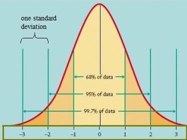
Prototype from University of Virginia
Creating a bell curve in Excel
Let's take a mutual example, and say we are analyzing exam results for a class of students. We volition be using a bell curve to measure exam results for better comparison.
We begin by computing the metrics to generate a normal distributed data which will generate our curve. Nosotros need to calculate:
- Mean (average) of the values.
- Standard difference of the values.
- 3-standard deviation limits for before and afterward mean.
- Interval value for usually distributed data points. This also requires a determination of the interval points. You lot tin select any number, only continue that in mind, more intervals hateful more than precision.
A quick notation earlier diving into the formulas. We used named ranges instead of cell references to make it easier to read the formulas. You tin find more than details about named ranges here: Excel Named Ranges
Metrics
Begin by calculating the mean and standard deviation of the information. You can use the AVEREAGE and STDEV.P functions to calculate the mean and standard deviation values respectively.

Next step is calculating the 3 standard deviation values to set the minimum and maximum values for the 99.7% of the data.
The 3 standard difference values can exceed the actual data prepare. This is a normal behavior that tin can occur frequently with smaller information sets.
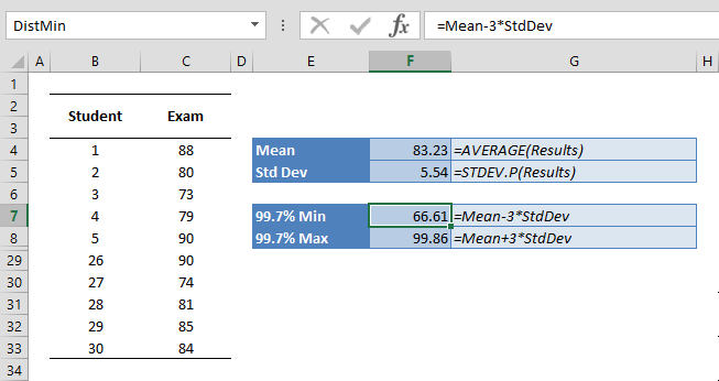
Minimum = 83.23 - three * 5.54 = 66.61
Maximum = 83.23 - 3 * five.54 = 99.86
After setting the minimum and maximum values for our bend, we demand to generate the intervals. The interval values will be the base for the ordinarily distributed values. To calculate the intervals, all you demand to do is to split up the area between the minimum and maximum values past interval count. In this example, nosotros set this to 20, simply yous can utilize a larger number to increment the number of information points.

Interval value = (99.85 - 66.sixty) / 20 = 1.66
Once the interval value is calculated, you lot can generate the data points. To do this, enter the minimum value in a cell. And then, right below the minimum value, enter the formula to add the interval value to the minimum. Here, nosotros used cell references (like as J4) which helps populate the information points easily up to the maximum value.

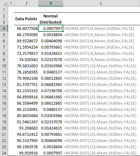
The next footstep is to summate the normally distributed values from the generated data points. Y'all tin can apply Excel'due south NORM.DIST office to generate these values.
Apply the populated data points as the starting time argument of the function. The hateful and standard deviation values are next arguments. End the formula with a Simulated Boolean value to use non-cumulative type of this function.
Nautical chart
Nosotros're almost done! Select the information points and normal distribution values, then insert an X-Y Scatter chart. Use the Scattered with Smoothen Lines version to create a bell curve in Excel.

The nautical chart may seem a bit off first. Let's see how you can make information technology wait better.
To change the championship of the chart, double-click on the title and update the name.
Adjacent, double-click on the Ten-axis and define minimum and maximum values from the Axis Options console to eliminate the white space on both sides. This will requite your chart a better bong shape. We prepare values that are a bit outside our data gear up. For example, 66 – 100 for values 66.xxx – 99.86.
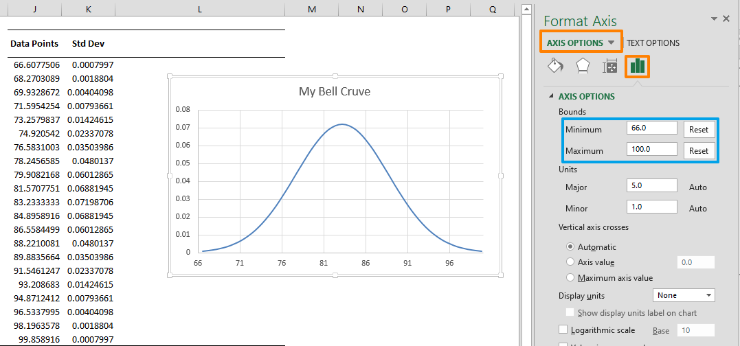
You can further enhance your chart by calculation the standard deviation values.


How To Create A Bell Curve In Excel With Data,
Source: https://www.spreadsheetweb.com/bell-curve-in-excel/
Posted by: orozcogerry1944.blogspot.com
0 Response to "How To Create A Bell Curve In Excel With Data"
Post a Comment